SCIN: Shield Current Induced Noise

SCIN: Shield Current Induced Noise

Jim Brown, Audio Systems Group

RaneNote 166, ©2003, 2004 Syn-Aud-Con

This article originally appeared in the Syn-Aud-Con Newsletter, 31, no. 4, 2003, and vol. 32, no. 1, 2004, reprinted here with permission.

• Causes
• Solutions

Introduction

My previous note focused on pin 1 problems as an open door for RF into audio equipment. But RF can also enter equipment on the signal conductor(s) if the equipment fails to block it with an effective low pass filter. RF is induced on a shielded balanced pair by at least three mechanisms:

• Imbalance in the magnetic coupling between the shield and the two signal conductors (Shield-current-induced noise).
• Voltage gradients resulting from imbalance in the capacitances between the two signal conductors and the shield.
• Coupling of the electric field through tiny openings in the shield.

In this note, we’ll focus on the first of those mechanisms.

For the same 1994 paper that introduced us to the “pin 1 problem,” subsequently published in the June 1995 issue of the Journal of the AES, Neil Muncy set up an experiment to study what happens when current flows on the shield of audio cable. With a power amplifier and output transformer driving the shield of audio cable with 100 mA sine and square waves at 60 Hz, 600 Hz, and 6 kHz, he measured the voltage induced on the signal pair. He called this voltage “shield-current-induced noise” (SCIN), noting that its amplitude was proportional to frequency and that it was due to the imbalance in magnetic coupling between the shield and the two signal conductors. He measured cables with a variety of shield constructions, and observed that cables with certain types of shield construction had much greater SCIN than others.

On the basis of Neil’s work, I had long suspected that SCIN was a major contributor to AM broadcast interference to audio equipment. Last year, I undertook research to prove it. I reported on that research at the Amsterdam AES this spring.

My experimental setup had to be different from Neil’s, because I wanted to measure SCIN from 10 kHz to at least 2 MHz (I eventually went to 4 MHz with that setup), and it’s hard to get more than about 100 kHz through even the best audio transformers. (I have recently devised another experiment showing that SCIN is alive and well to at least 300 MHz, and will report on it at the AES in NY in October).

For the 4 MHz tests, I drove the shield of the test cable end-to-end using a 50Ω RF generator, and mea-sured the current by connecting an RF voltmeter across a 2.5Ω resistor in series with the shield. Neil used a constant current of 100 ma, which he considered representative of what often flows in the shield of audio cable. He could easily produce that current and hold it constant with the power amplifier. The RF generator is capable of a lot less current, especially when driving the inductance of a long cable, and the available current varies widely with frequency and the length of the cable because the generator is a much higher impedance source. To get more current between 10 kHz and about 250 kHz (increasing the sensitivity of the measurement), I used an old vacuum-tube Hewlett Packard audio generator. I also knew wavelength effects and resonance in the cable would introduce errors, so I measured four lengths of cable -- 125 ft, 50 ft, 25 ft, and 10 ft. Figures 1 and 2 show the test setup.

Figure 1. The SCIN test setup.

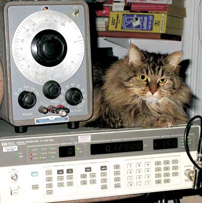
Figure 2. The HP 200CD audio generator was used for most data below 250 kHz -- the HP 8657A at the higher frequencies.

A variety of cables were tested, each given a descriptive identifier to aid in interpreting the data. The first letter indicates shield construction -- B for braid, F for foil, S for spiral shield, CP for conductive plastic. Letter D indicates the presence of a drain wire. Q indicates quad construction. Letter A indicates an analog cable, a second letter D indicates a digital cable. A number indicates another cable of the same generic type.

Neil’s research, conducted only at audio frequen-cies, showed that foil/drain-shielded cables had the worst SCIN performance, while braid-shielded cables were about 30 dB better. My research shows that braid-shielded cables maintain this advantage to at least 2 MHz, but gradually begin to lose it above that frequency. My more recent work shows that the braid cables are still better to at least 7 MHz and about the same as foil/drain construction at 14 MHz. By 28 MHz, the foil/drain cables are better.

Figure 3 shows that all the foil/drain cables perform similarly, with the exception of FDA1 and FDA2, which had markedly less SCIN. But cable BF, a low cost foil/braid-shielded cable with no drain wire, custom manufactured in Brazil for Dave Distler at the suggestion of Ray Rayburn, had far superior SCIN performance. In fact, Figures 8 and 9 show that the SCIN of BF was on a par with BA, a premium braid-shielded cable!

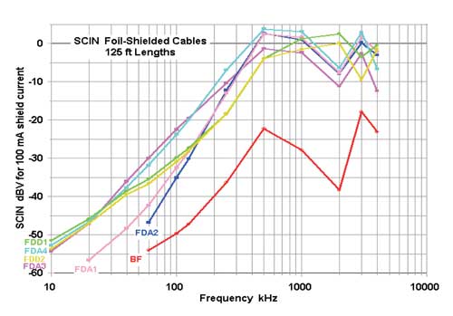
Figure 3. Data for 125 ft lengths of the foil-shielded cables.

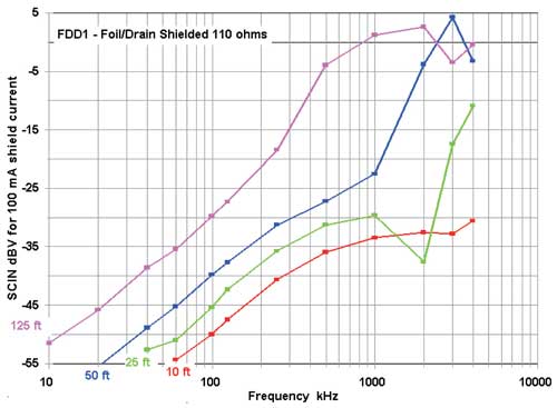
Figure 4. A typical, good quality, foil/drain shielded cable, normalized to 100 mA current, but not normalized for length.

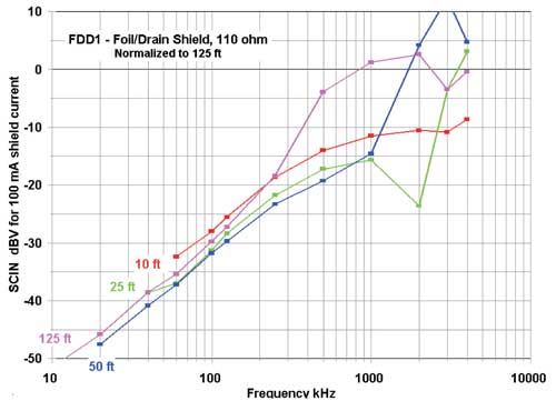
Figure 5. The same data as in Figure 4, normalized both for 100 mA shield current and to a length of 125 ft.

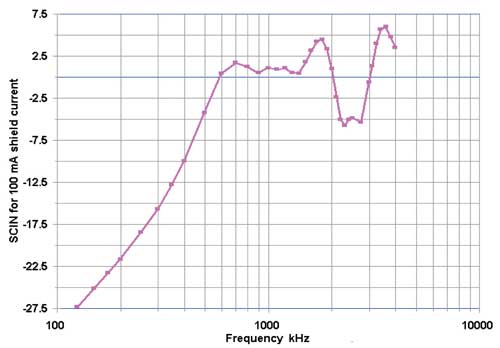
Figure 6. Data taken at closer spaced points for the 125 ft length of cable FDD1.

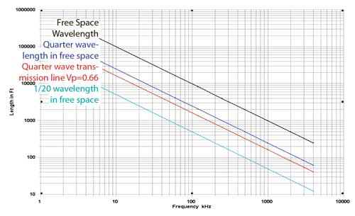
Figure 7. Wavelength and frequency relationships.

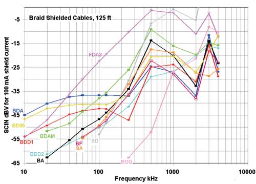
Figure 8. The braid-shielded cables, and one foil-shielded cable (FDA3) for comparison.

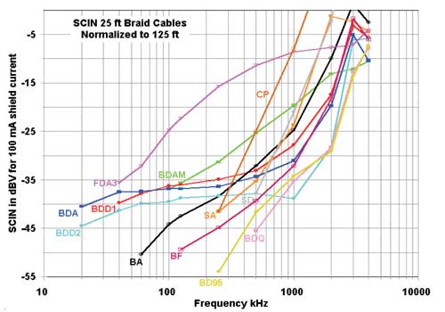
Figure 9. The braid-shielded cables, and one foil-shielded cable (FDA3) for comparison.

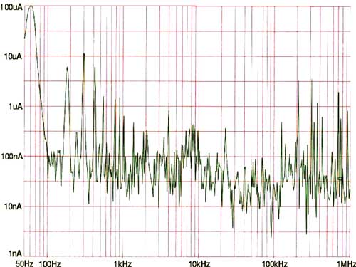
Figure 10. The noise spectrum of a typical power line. (Courtesy of Bill Whitlock)

The data for SCIN in cables is significantly more complex than is obvious in Figure 5, which shows data taken in increments of one octave. The more closely spaced data points of Figure 6 clearly show multiple resonance and wavelength effects, but the noise is clearly increasing linearly with frequency below 500 kHz. Bill Whitlock has shown that the first peak, around 700 kHz for this cable and this length, is the resonance between the series inductance of the shield and the cable’s capacitance. Some of the other peaks and dips are related to the wavelength of the cable based on its behavior as a transmission line. All of these effects will scale with the length of the cable. That is, short cables will exhibit a linear increase of SCIN to a higher frequency, and resonances will move higher in frequency.

Just as acoustic standing waves are established in rooms, electrical standing waves occur on any cable where radio frequency voltage and current are present. The result is that the cable will show resonance effects based on its length. The cable lengths tested here exhibited multiple transmission line-related resonances, and, as we’ll learn later, they will be particularly effective as receiving antennas for at those resonant frequencies. See the ARRL Handbook and ARRL Antenna Book to learn about transmission lines.

All of the cables shown in Figures 8 and 9 are designed for portable use (except for FDA3, shown for comparison). BA is a popular, high quality, braid-shielded cable, SA an excellent European cable with a double spiral shield. BDAM is a high quality miniature analog cable that is a single pair of a family of snakes, and is approximately the same size as FDA3 and FDD1. Types BA, SA, and FDA3 were also measured by Muncy.

When studying the data, it helps to think about what potential interference (noise) sources are typically present in any given part of the spectrum. The standard AM broadcast band extends from 540 – 1,700 kHz throughout most of the world; there are also broadcast, business, and scientific users of the spectrum between 50 kHz and 500 kHz. In addition, the spectrum between about 10 kHz and 1 MHz is full of noise from motors, lighting equipment, switching power supplies, control signals for clock systems, etc. Harmonics of power-related distortion and switching transients are also present.

Figure 10 shows a typical power line noise spectrum. Filter capacitors will couple all of the noise onto the ground, which in sets up noise current in the shield of audio cables running between widely separated points. SCIN will couple this noise onto the signal pair!

Here are some important conclusions that can be drawn from a study of the data.

1. Cables BD95, BDD1, BDA are of similar size and quality to BA, yet BA has much less SCIN below about 250 kHz. The difference is the presence of a drain wire in all but BA, which degrades the uniformity of distribution of current in the shield. The data clearly shows that the net effect of a drain wire is to significantly degrade SCIN performance below about 500 kHz.
2. BDAM and FDA3 are of very similar size, yet BDAM has 12-15 dB less SCIN because the braid component of its shield carries a higher proportion of the shield current than does the foil of FDA3. In fact, the ratio of their SCIN performance is very close to the inverse of the ratio of the resistance of the drain wire to the total resistance of the shield! That is, the strength of the SCIN is proportional to the percentage of the total shield current that flows in the drain wire.
3. Cable BDQ ( a Gepco product) exhibited excellent SCIN performance. A short sample (all I had) of another well known quad cable did not measure nearly as well. [Quad construction is not without its drawbacks -- star quad cables have far greater capacitance between conductors than conventional cables. Dennis Bohn has observed that placing an excessive capacitive load on the output stages of microphones and other audio equipment causes distortion of high frequency transients.]
4. Braid shields are far superior to foil shields with respect to their ability to reject interference below 4 MHz.
5. As we will learn next, a foil/braid shield is good at all frequencies!
6. SCIN will cause RF to be coupled to the signal pair, so audio equipment must include good low-pass filtering to reject it.
7. Extending the bandwidth of audio gear much beyond 100 kHz in a quest for ideal phase response is an invitation to RF interference.

Figure 11. Wire topology.

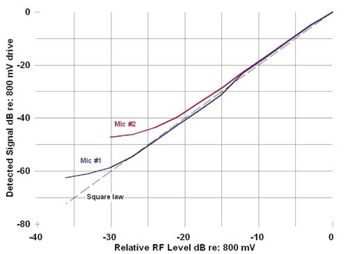
Figure 12. Square law response of two typical microphones.

Induced Cable Current

One of the obvious questions is, “How much current can there be on the shield of audio cables in a given installation? Research by Neil Muncy and others suggests that 100 mA of power-related current (i.e., 50/60Hz and harmonics) is not uncommon where the source of the current is the power system within buildings. Muncy’s 1994 SCIN measurements and John Wendt’s “Hummer” tester for pin 1 problems, both used this level of current. But how much current might an AM broadcast transmitter induce in the mic cable shields running through the loft of a wood frame church?

To answer that question, I devised a set of experiments using 125 ft lengths of mic cable connected to a Hewlett Packard 3586C Selective Level Meter. The 3586C is essentially a calibrated voltmeter in the form of a radio receiver that can tune to any frequency between a few kHz and 32 MHz. It can also measure the frequency of a signal within that range to an accuracy of about 0.1 parts/million. Data were taken at two locations. Location #1 was a wood frame pagoda in an open park where Ron Steinberg (who assisted with the measurements) had installed a small sound system. It is within about 4 miles of three high power AM broadcast transmitters. The 125 ft length of mic cable was supported about 7 ft above moist earth by low limbs of small trees and connected to the 3586C, which was set up in the pagoda. Location #2, roughly 20 miles from the first, was the 120 year old wood frame house that also serves as my office and lab. Here, the same 125 ft length of mic cable ran from one end of the third floor, around the house to my laboratory at the front of the second floor. In both cases, the 3586C was powered from a grounded 120 VAC outlet.

At each location, the cable shield was connected to the center conductor of the 50Ω coaxial input of the 3586C, and the voltage produced by the carrier of several dozen AM broadcast stations was measured. Ohm’s law then told us the current for each station. The FCC’s website lists the locations, transmitting antenna characteristics, and power level of each station.

All of the stations measured were within about 40 miles of the measurement location (but each was at a different distance and azimuth) so their propagation was by ground wave. In the far field, the drop in field strength of a ground wave signal has two principal components that are additive -- inverse square law, plus a term due to the loss caused be the current flowing in the earth that varies with the resistivity of the soil and the frequency of the signal. As part of their AM broadcast regulations, the FCC has long published empirically determined families of curves that allow the ground wave field strength to be predicted with good accuracy to more than one hundred miles. These curves were used to take the data measured for each station and estimate the current that would flow in the same cable if it were only 1 mile from the transmitter and at the same azimuth.

AM broadcast antennas are always vertical, typically one quarter wave tall. The entire tower is the antenna. Some (mostly the highest power stations) use half-wave or 5/8-wave tall antennas, producing a field strength in the horizontal plane that is respectively 1.9 or 3.2 dB greater than a quarter wave antenna (as with loudspeaker directivity, you don’t get something for nothing -- the gain is at the expense of reduced output at higher angles, but with radio, that’s good). Most (but not all) AM broadcast stations are omnidirectional during daylight hours but switch to directional operation at night; some are always omnidirectional, and some are directional at all times. Several different power levels are used. The highest power stations use 50 kW to cover several states; others operate at 10 kW, 5 kW, 1 kW, or even 250 W to cover smaller areas.

My measurements showed the 125 ft cable shield (antenna) will typically see about 5 mA at 1 mile from an omnidirectional 50 kW station with the taller antenna. Currents were typically 1.5 mA and 0.75 mA for 5 kW and 1 kW, respectively. The shield current will likely vary by ±10 dB depending on the orientation, height, and geometry of the receiving antenna and another +10/-12 dB based on any directionality of the transmitting antenna. Thus typical shield currents on the order of 1-20 mA should be expected 1 mile from a 50 kW transmitter in a 125 ft mic cable that is unshielded by conduit or building steel, 0.5-10 mA at 1 mile from a 5 kW transmitter, and 0.2-2 mA at 1 mile from a 1 kW transmitter. These data, although carefully measured, can hardly be taken as precise. They will, however, give us some idea of the general order of magnitude of the RF signal that might be expected. More important, circuit designers ought to be applying these estimates to the SCIN data to predict how much RF immunity their equipment might need in the real world!

When diagnosing and eliminating RF interference in systems, it is quite helpful to realize that a relatively small reduction in RF signal level can make a large reduction in the audible interference. In other words, a reduction in RF level of only 10 dB will reduce the audible interference by 20 dB. In practice, this means that we may not need to go after RF interference with a sledge hammer (i.e., a very costly solution), but rather may be able to use much simpler ones. I’m currently doing some research on RFI solutions, and hope to be able to report on them before long.

Figure 14 shows the results of testing a very good product, the Sound Devices Mix Pre. Ron Steinberg loaned me this unit for the condenser mic RF testing I described this past spring, and it’s the most “bullet-proof” product I’ve tested so far. The red curve shows the detected RF when you drive pin 1 of channel 1 and listen to channel 1. The blue curve shows the crosstalk you hear when you inject at the same point, but listen on channel 2. This sort of crosstalk happens with virtually every piece of gear I’ve tested, and the reason should be obvious -- the RF is getting injected into the circuit board via a common impedance, which in turn adds it at multiple points in the signal chain. The peaks and dips in the response are probably the result of the addition of detection from multiple points in a circuit as the phase and amplitude relationships between those detected signals vary with frequency.

Figure 15 shows test results for a small mixer in a family notorious for picking up AM radio stations. The mixer shown in Figure 16 was designed in response to a chorus of complaints, and it fixed the problem in most installations. But while the mixer of Figure 16 is at least 40 dB better on the AM broadcast band, it is at least 30 dB worse in the VHF spectrum, and was thus unusable for my microphone testing in downtown Chicago!

Test results for a small rack mount compressor/limiter are shown in Figure 17. In this unit, the pin 1 problem is at it’s worst between 20 and 50 Mhz -- it probably makes a wonderful CB radio! The ¼" connectors used for inputs and outputs have plastic bushings that insulate them from the chassis. This is a fixed threshold unit, and the pin 1 problem is so severe the rectified audio from the pin 1 test is hitting that threshold! When I spoke with the designer of this unit a few years ago at AES about the pin 1 problem, he loudly proclaimed that Whitlock guy didn’t know what he was talking about.

Last summer, I talked about pin 1 problems in microphones, concurring with Neil Muncy’s hypothesis that the majority of RF susceptibility in audio gear was the result of a pin 1 problem. I’ve always wanted to devise a method of measuring pin 1 susceptibility of audio gear. Figure 13 shows the setup I settled on. In effect, all I’ve done is replace the wall wart in John Wendt’s hummer with an RF generator and cooked up a way to plot the result using audio gear that I already owned. I used the same generator I used for the SCIN measurements, but any good RF generator will work.

Figure 13. A test rig for RF pin 1 problems.

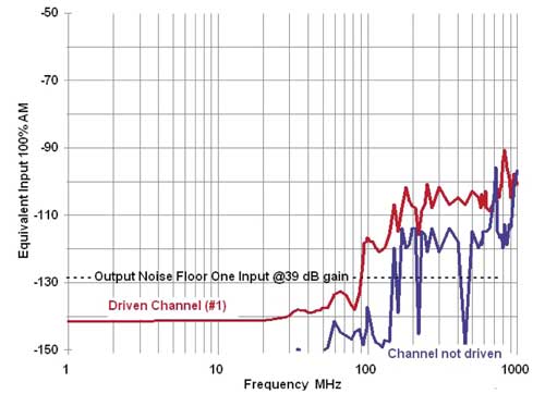
Figure 14. The pin 1 test for a very good product

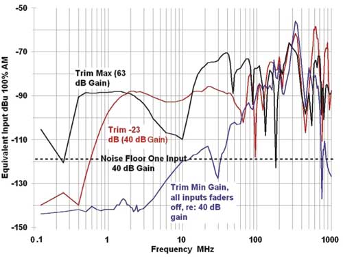
Figure 15. The pin 1 problem in a small mix console known for picking up AM radio stations

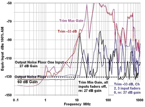
Figure 16. The console that “fixed” the problem in many installations (but not at VHF!)

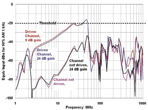
Figure 17. A dual compressor/limiter with a serious pin 1 problem

I’ve also devised a method for injecting differential-mode RF onto the signal pair in much the same way that SCIN would do it in that typical church. As you might guess, I’ve also applied both of these techniques to microphones, and have measured many of those I field tested last winter. A detailed discussion of the test setups and loads of data are included in the two papers I presented to the AES in New York this fall. They are available from the AES, though not on the website yet.

And this footnote: Russ O’Toole called me the other day to tell me about a contractor whose work he was inspecting, who insisted on un-twisting several inches of twisted pair cables before connecting it to equipment. He was looking for something in print saying that this was a bad idea. Well, here it is!

Cable Shields

Nearly all interference below a few hundred kHz is magnetically coupled. Cable shields provide almost no magnetic shielding in this range. On the other hand, twisting is very effective against magnetically coupled interference. In general, rejection of magnetic fields is proportional to the number of twists per unit length (called the “lay”) and the uniformity of the twisting. Structured cable (CAT 5, etc.) achieves its relatively high noise rejection by virtue of a high twist ratio. For a century, virtually all telephone lines have run for miles on unshielded twisted pairs.

In his seminars, Neil Muncy demonstrates the importance of twisting by running a very long string of mic cables around a lab and using them to connect a mic in an acoustically isolated container to a small mixer/amp that feeds loudspeakers for the audience with a lot of gain. He then takes a tape eraser (for you youngsters, that’s a big coil driven by the power line to generate a big 60 Hz magnetic field to erase magnetic tape) and moves it along the mic cable. No hum is heard with the demagnetizer anywhere along the cable except at the connectors, where it can get fairly loud. Why? The twisting is interrupted at the connectors!

Twisting is also important for good RF rejection. It’s quite common for untwisted parallel cables (zip cord) to couple RF into equipment when used as loudspeaker cable, and for the interference problems to be solved when it is replaced by an unshielded twisted pair. Yet another reason to avoid most high futility loudspeaker cables! [I never cease to be amazed at how little real science the purveyors of all that pseudo-science actually understand. After one of my rep friends went through the “training” sessions held by the manufacturer of one of the better known of these product lines, he asked them for some data he could show his technically inclined clients to back up their claims. They responded that they had no such data and no gear to measure it, but they would appreciate any data he could provide!]

Cable shields are effective against electric fields, and can be quite important where there is RF interference. If the cable is short as compared to the wavelength of the interference, the shield only needs to be connected at the sending end. If the cable is much longer than about 1/10 wavelength, the shield needs to be as continuous as possible and connected at both ends. As noted earlier, the ideal connection is a concentric one. Next best is the shortest practical pigtail.

So, to summarize, the “right” way to terminate balanced cable, whether for audio or data, is to maintain the twisting as carefully as possible right to the point where it enters equipment (ideally there should be “zero length” of untwisted cable). If the shield is to be terminated, there should be either a concentric connection or the shortest possible pigtail, and it should go straight to the shielding enclosure of the equipment. If the connection is needed to shield against VHF RF but needs to be interrupted at lower frequencies to prevent shield current, a capacitor should be used in series with the shield connection (also with very short leads or a concentric connection), and only at the receive end.

"SCIN: Shield Current Induced Noise" This note in PDF. (4M)